Crypto Market Cap
Top 20 coins as a donut, with the 21st slice the rest of the market. Switch between circulating and fully-diluted valuation, compare data sources, and click coins to exclude them from the total.
US Stock Market Cap
The top ~1000 US-listed companies by market cap — live from Yahoo, categorized by sector. Choose a Top-N or a sector to view, click any stock to pull it into a selection pie, and compare against FMP.
Market Sentiment
Real-time crowd sentiment from StockTwits and Reddit — bullish vs. bearish signals scored by VADER + community tags.
Stock Analysis
Historical price chart with SMA overlays and key fundamentals for any US-listed stock — type a ticker and pick a time range.
ETH Validators 💎
Live Ethereum beacon chain validator stats — active validators, queue sizes, total staked ETH, staking APR, and network participation rate. Data via beaconcha.in, refreshed every 60 seconds.
Deuces Wild Bonus Poker
All 2s are wild. Edit the payoffs, pick your 5 dealt cards, hold what you want, then choose your draw cards.
Pay Table — payout at 5-coin max bet
Deck — click cards to choose 2 = wild
Solitaire
Klondike. Click a card to pick it up, then click where to move it. Double-click a card to send it to a foundation. Click the stock (top-left) to deal.
Polymarket 🔮
My filtered Polymarket — add the sports you care about and it shows the next game for each, winner only. Sign in with Phantom to trade. Auto-refreshes every 30s.
FIFA World Cup 2026 — Bracket Predictor 🌍
48 teams, 12 groups, one trophy across the USA, Canada & Mexico. Predict every group scoreline — the 8 best third-placed sides advance automatically — then click your way from the Round of 32 to a champion and share your bracket with a link. Kick-off: 11 Jun 2026.
Premier League 2026-27 — Season Predictor ⚽
Drag the 20 clubs into your predicted final table, set your bonus picks, then save or share. Kick-off: 22 Aug 2026.
EFL Championship 2026-27 — Season Predictor 🏆
Drag the 24 clubs into your predicted final table. Top 2 go up automatically, 3rd–6th into the play-offs, bottom 3 down. Kick-off: Aug 2026.
EFL League One 2026-27 — Season Predictor 🥉
Drag the 24 clubs into your predicted final table. Top 2 go up automatically, 3rd–6th into the play-offs, bottom 4 down. Kick-off: Aug 2026.
EFL League Two 2026-27 — Season Predictor 🎖️
Drag the 24 clubs into your predicted final table. Top 3 go up automatically, 4th–7th into the play-offs, bottom 2 drop to the National League. Kick-off: Aug 2026.
Claude Code Usage 🤖
My live Claude Code subscription usage, read straight from this server's own logs — a public look at how much API-equivalent value a flat-rate plan delivers.
AI Market Map 🧠
A top-model comparison across the leading US and Chinese labs, plus the companies that power the AI industry grouped by the layer of the stack they play in — from foundation models down to the silicon. Search or filter by layer.
Security & Network 🛡️
Live server health — bandwidth, latency, connections, traffic, top IPs, and auto-flagged scanners. Refreshes every 5–10s.
Integrations 🔗
Manage third-party account connections. All tokens are stored server-side only and never sent to the browser.
Photos 📸
Browse your Google Photos library — albums, photos, and videos. Owner only.
Mail ✉️
Inbox for me@patd.dev — mainly account verification emails. Owner only.
🧠 The AI Debate
Working notes — building up from the very first artificial neuron toward modern models, one historical step at a time. Alongside the technical timeline, this page also tracks the major philosophical critiques of AI as they arise, and checks each one against how the field actually developed — some proved right, some wrong, some are still open.
1888 — Santiago Ramón y Cajal: The Neuron Doctrine
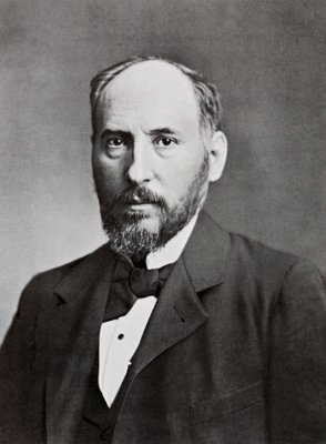
Before anyone could model "a neuron" as a discrete unit, someone had to prove neurons ARE discrete units.
Using Golgi's newly-invented staining technique, Cajal produced meticulous, detailed drawings showing the nervous system is made of separate, individual cells — neurons — with tiny gaps between them, not one continuous connected web as the rival "reticular theory" held. This became known as the neuron doctrine. Ironically, Cajal shared the 1906 Nobel Prize in Physiology or Medicine with Camillo Golgi himself, despite the two holding directly opposing views about how the nervous system worked.
This is the biological prerequisite for literally everything else on this page: McCulloch & Pitts' 1943 model (the very next relevant entry) treats a neuron as one discrete computational unit with its own inputs and output specifically because Cajal had already established, decades earlier, that this is biologically real — not a simplifying assumption, but an accurate reflection of actual nervous system structure.
1921 & 1953 — Ludwig Wittgenstein: Logic's Foundations, Then Its Own Best Critique philosophical throughline
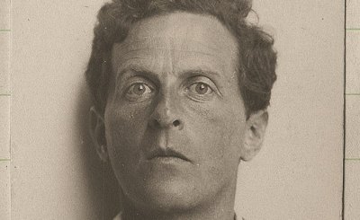
Predates AI as a field entirely — but supplied both its logical foundation and, decades later, its own deepest critique.
Wittgenstein appears twice in this story, arguing with himself across three decades. In 1921, his Tractatus
Logico-Philosophicus laid out the systematic truth-table method for propositional logic — proposition 5.101
gives the general formula for the number of possible truth-functions of n inputs, 2^(2^n), the exact
formula behind the "16 possible 2-input functions, 256 possible 3-input functions" discussion already covered on
this page. This is squarely in the tradition that later enables McCulloch-Pitts, Boolean logic gates, and formal
symbolic computation generally — the young Wittgenstein believed logic could exhaustively capture how language
pictures the world.
Then he spent his later career dismantling that picture. In the posthumously published Philosophical Investigations (1953), Wittgenstein rejected his own earlier framework — arguing that meaning doesn't come from fixed logical correspondence between language and world, but from use within social practices ("language games," "forms of life"). His "rule-following paradox" makes a very specific, sharp claim: no finite set of explicit rules can ever fully determine its own correct future application — any rule can be interpreted to fit multiple different continuations, so rule-following ultimately rests on shared practice and training, not on the rules themselves being self-interpreting. This is a direct philosophical ancestor of Dreyfus's critique below, decades before AI existed as a field to critique.
📄 Tractatus Logico-Philosophicus (1921), Project Gutenberg
1943 — Warren McCulloch & Walter Pitts
The first mathematical model of a neuron. Not trained — hand-designed.
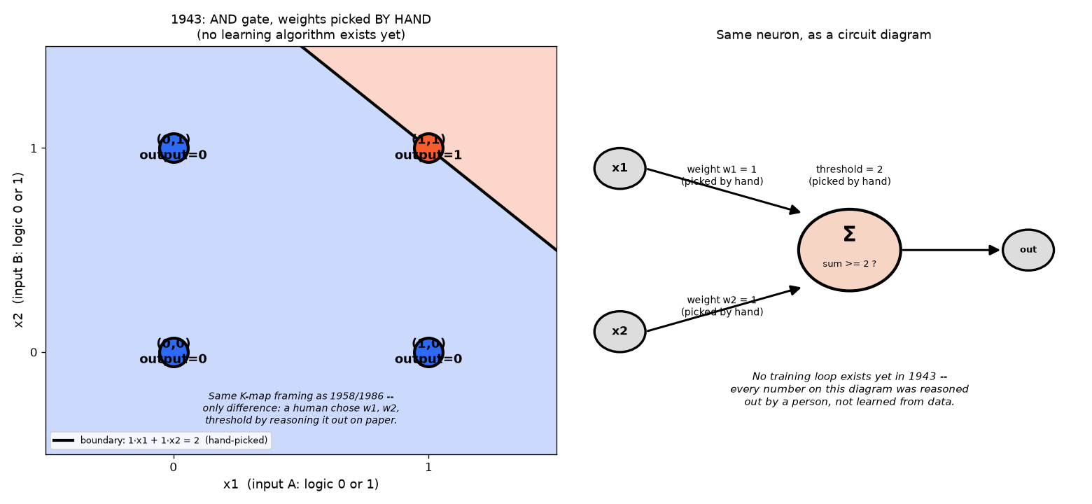
McCulloch (a neurophysiologist) and Pitts (a self-taught logician) formalized what was already known experimentally about real neurons — Adrian's 1920s recordings had shown neurons fire in an all-or-nothing way, and there's a real, measurable voltage threshold that must be crossed before a spike fires. They turned this into pure math: multiply each input by a fixed, hand-chosen weight, sum them, and fire (output 1) only if the sum clears a threshold. No learning algorithm existed yet — the weights were picked by hand.
A single neuron built this way can compute AND, OR, and NOT just by choosing different weights/thresholds. It cannot compute XOR — no single straight-line boundary can separate that pattern, a limit that would matter enormously 26 years later.
Reading the diagram below, in EE terms: same Karnaugh-map-style plot and circuit diagram
as every later entry on this page — the only difference from 1958 onward is that here, a human reasoned out
w1=1, w2=1, threshold=2 on paper. There's no training loop yet to find these numbers automatically.
📄 A Logical Calculus of the Ideas Immanent in Nervous Activity (1943)
1949 — Donald Hebb: "Neurons That Fire Together, Wire Together"
The conceptual ancestor of every learning rule on this page — proposed before anyone had built a machine that could actually learn.
Hebb's book The Organization of Behavior proposed that learning happens through changes in synaptic strength: when one neuron repeatedly helps fire another, the connection between them gets stronger. His own summary, more precise than the popular one-liner: "when an axon of cell A... repeatedly or persistently takes part in firing [cell B], some growth process or metabolic change takes place... such that A's efficiency... is increased." Note this is purely correlational — cells that tend to activate together get a stronger connection — with no notion of a "correct answer" to compare against.
This is a genuinely different idea from Rosenblatt's 1958 perceptron rule (which arrives 9 years later): Hebb's rule strengthens connections based on co-activation alone, while the perceptron rule specifically corrects weights based on being wrong against a known target. Hebbian learning is the conceptual seed — a synapse's strength is not fixed, it changes with experience — that every error-driven learning rule on this page (perceptron, backprop) later sharpened into something usable for training toward a specific correct answer.
1950 — Alan Turing: "Computing Machinery and Intelligence"
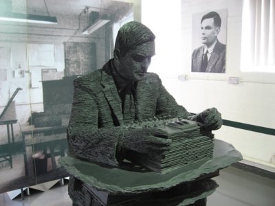
Not a neuron model at all — a completely different question: how would we even know if a machine could think?
Turing sidestepped the philosophically messy question "can machines think?" (he considered it too vague to be useful) and replaced it with something practical: the Imitation Game, now known as the Turing Test. If a human judge, holding a text conversation with both a person and a machine, cannot reliably tell which is which, the machine should be considered functionally intelligent — for practical purposes, regardless of what's "really" happening inside it.
This reframed the entire field around external behavior rather than internal experience — a genuinely different axis from McCulloch-Pitts' "how do you build a computing neuron," and one that's still argued about today (this is the same underlying question as the "stochastic parrots" debate about whether large language models "truly understand" anything, which we discussed earlier this session).
📄 Computing Machinery and Intelligence (1950), Mind
From Source Code to Hardware: a Real Compilation Pipeline
Turing is called the father of computer science for a reason — this whole pipeline is downstream of his theoretical work on what a "computer" fundamentally is and can do.
Turing's abstract "Turing machine" (from his earlier, even more foundational 1936 work, before the
Turing Test above) is the theoretical model underlying every real computer since — a precise definition
of what it means to "compute" something mechanically, step by step. Everything below is that abstraction
made concrete: all of this session's Python (and every neural network on this page) eventually becomes
real hardware instructions the same way any program does. Rather than describe that abstractly, here's an
actual simple adder function, compiled for real on this machine with gcc 13.3.0, showing
genuine output at every stage — not a fabricated example:
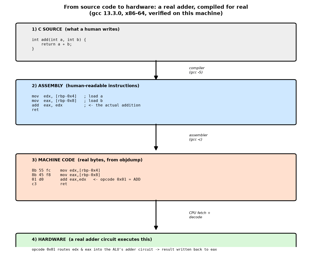
Reading the pipeline: the compiler turns C into human-readable assembly (stage 2) —
note the actual work is just one line, add eax, edx; everything else is just moving numbers
into and out of registers. The assembler then turns that into raw bytes (stage 3) — 01 d0 is
the literal machine code for that add instruction; 0x01 is x86-64's opcode for "add," and
d0 encodes which two registers to use. When the CPU fetches and decodes that byte, it
physically routes the two register values into the ALU's adder circuit — real transistors doing real
binary addition, the hardware endpoint of every abstraction on this page.
This is the same relationship as the McCulloch-Pitts neuron's sum ≥ threshold comparator
from the very first entry above: a mathematical operation described in software ultimately bottoms out as
a specific, physical arrangement of logic gates — whether that's a general-purpose CPU's ALU decoding an
opcode, or a dedicated neural-network ASIC with a hard-wired MAC (multiply-accumulate) unit built to do
nothing but that one operation, as fast as possible.
1952 — Hodgkin & Huxley: The Actual Circuit Model of a Neuron
Genuinely an EE-relevant entry — this is a literal circuit model (capacitor + variable resistors + batteries) of a real biological cell.
Using the (unusually large, easy to experiment on) squid giant axon, Hodgkin and Huxley worked out the actual ionic mechanism behind a neuron's electrical spike — the "action potential" already referenced back in the 1943 entry's mention of Adrian's 1920s all-or-nothing recordings, now given a precise, quantitative explanation. Their model represents the cell membrane as a capacitor, and each type of ion channel (sodium, potassium) as a variable resistor in series with a battery representing that ion's equilibrium voltage — four coupled differential equations describing exactly how these conductances change with voltage and time to produce a spike. This won them the 1963 Nobel Prize, and their equations are still the standard starting point for computational neuroscience today.
Where this fits on this page: McCulloch-Pitts' 1943 neuron reduces "does it fire" to a simple threshold comparison — accurate as a first approximation, but Hodgkin-Huxley is what that threshold actually looks like at the level of real ion channels opening and closing. Every artificial neuron on this page is a drastic simplification of this real circuit, trading biophysical accuracy for something trainable at scale.
The nonlinearity goes deeper than just the final spike, too. The Hodgkin-Huxley equations themselves are explicitly nonlinear — each ion channel's conductance depends on voltage through gating variables that follow their own nonlinear (sigmoid-shaped) curves, not a simple linear relationship. But real neurons are nonlinear in an even richer way than that single spike-or-not decision suggests: a neuron's dendrites (the branching input structure feeding into the cell body) aren't just passive wires summing up inputs linearly before reaching a single threshold — they contain their own voltage-gated channels, capable of local, nonlinear interactions within different branches of the same neuron, before any signal even reaches the main spike-generating threshold. Some real dendritic branches have been shown experimentally to compute something logically similar to AND or even XOR-like operations locally, using nonlinear dendritic interactions — meaning a single biological neuron may be capable of a small amount of the same "multiple comparator lines combined" computation that our artificial network needed two entire neurons to achieve back in the 1986 XOR entry. Every artificial neuron on this page — including the ones inside today's frontier transformers — collapses all of this rich, nonlinear, spatially-structured dendritic computation down to one linear weighted sum plus one simple nonlinear activation function. That's a real, deliberate loss of biological complexity in exchange for something trainable at massive scale, not evidence the artificial version is a faithful copy of the biological original.
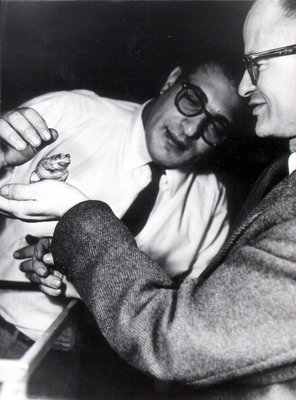
1956 — The Dartmouth Conference
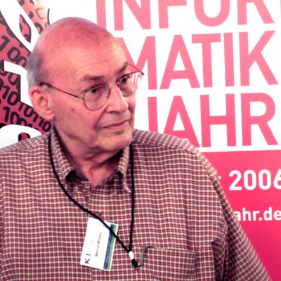
(1 of 4 organizers)
Where "Artificial Intelligence" was named as a field — no working system, just a founding event.
John McCarthy, Marvin Minsky (yes — the same Minsky from the 1969 critique below), Claude Shannon (the same Shannon whose 1937 thesis first showed Boolean logic could be built from relay circuits), and Nathaniel Rochester organized a summer workshop at Dartmouth College proposing that "every aspect of learning or any other feature of intelligence can in principle be so precisely described that a machine can be made to simulate it." That sentence is literally where the term "Artificial Intelligence" was coined.
No breakthrough system came out of the workshop itself — its real significance is that a scattered set of related ideas (cybernetics, information theory, automata theory, McCulloch-Pitts-style neuron models) got a single shared name and identity as one field for the first time, which is what let it start attracting dedicated funding and researchers.
📄 A Proposal for the Dartmouth Summer Research Project (1955)
1958 — Frank Rosenblatt's Perceptron
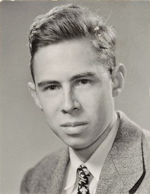
The real innovation: a neuron that changes its own weights from data.
McCulloch-Pitts neurons had to be hand-designed by a person who already knew the answer. Rosenblatt's breakthrough — built at Cornell, and physically realized as the Mark I Perceptron machine in 1960 (400 photocell "eyes" wired to adjustable resistors standing in for weights) — was a genuinely new idea: a simple rule for the neuron to correct itself, using only its own mistakes, with no human manually tuning anything.
The rule is almost embarrassingly simple: show it an example, let it guess, and if it's wrong, nudge every weight a little in the direction that would have made it right. Repeat.
Reading the diagram below, in EE terms: x1 and x2 are the two binary logic inputs (0 or 1)
feeding the neuron — think of them as two digital signal lines. The neuron computes a weighted sum
(a summing junction, like a summing op-amp: x1·w1 + x2·w2 + bias) and compares that sum
against zero, exactly like a comparator with its reference tied to ground: sum ≥ 0 → output HIGH (1),
sum < 0 → output LOW (0). The left plot is just a Karnaugh map for 2 inputs, but instead
of hand-circling groups of 1s, the boundary between regions is drawn by that comparator equation directly —
the black line is every point where the sum is exactly zero. The right diagram is the
exact same math, drawn the way a circuit/network diagram usually looks, with the real learned weight and
bias values labeled on each connection.
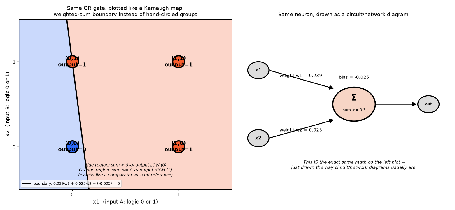
Where do 0.239 and 0.025 actually come from? This diagram now runs the real 1958 learning
rule to produce them — starting from small random weights, then repeatedly applying
new_weight = old_weight + learning_rate × error × input against the OR truth table until every
case is answered correctly. Notice the two weights aren't equal, and that's the honest, important part:
the perceptron rule only nudges a weight when its corresponding input was actually 1 for that example (the
rule multiplies by input, so a 0-input contributes no correction that round). Depending on the
random starting point and which examples happen to correct the weights first, training can validly land
on many different final lines that all correctly separate OR's four points — 0.239/0.025 here isn't "the"
answer, just one valid one this particular run converged to. Re-running with a different random seed would
converge to different (but equally correct) numbers.
This is the moment "training a model" — as opposed to "designing" one — was born. Every model we've run since (including the frontier ones) is a direct descendant of this same core idea: guess, measure the error, adjust the weights, repeat.
📄 The Perceptron: A Probabilistic Model (1958), Psychological Review
1959 — Arthur Samuel's Checkers Program parallel branch, not part of the neuron lineage
Coined the term "machine learning" — using a completely different technique from neurons.
Samuel, at IBM, built a program that played checkers against itself thousands of times, using a scoring function (an evaluation of how good a board position looks) combined with a search over possible future moves, and refined that scoring function based on which choices led to wins. Not a neuron, no weighted sum, no threshold — a different lineage entirely, based on game-tree search and self-play. It's the paper that literally coined the term "machine learning."
In a famous 1962 exhibition match it beat a strong human amateur player, generating major press coverage of "thinking machines" — a very public, concrete proof that a computer really could improve its own performance from experience, not just execute a fixed program.
1959–1962 — Hubel & Wiesel: The Visual Cortex's Hierarchy
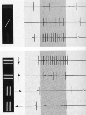
The direct biological inspiration for the CNN entry later on this page — this is not a loose analogy, it's a documented, named lineage.
Recording directly from neurons in a cat's visual cortex, Hubel and Wiesel discovered two distinct cell types: "simple cells" that respond strongly only to a specific, narrow orientation of edge (a vertical line, say) at one specific location, and "complex cells" that respond to the same kind of edge across a range of locations — achieving that flexibility, they proposed, by pooling input from many simple cells with the same orientation preference but different positions. This revealed the visual cortex as hierarchically organized: simple, local feature detectors feeding into progressively more complex, more position-tolerant ones. This won them the 1981 Nobel Prize.
This is a direct, documented inspiration, not just a loose parallel: Kunihiko Fukushima explicitly built his 1979/1980 Neocognitron — the direct architectural ancestor of the CNN entry later on this page — as a computational model of exactly this simple-cell/complex-cell hierarchy. The Neocognitron's local receptive fields and pooling layers are a direct translation of Hubel & Wiesel's biology into a trainable architecture, which LeCun's LeNet later refined with backpropagation.
1965 — Lotfi Zadeh's Fuzzy Logic parallel branch, not part of the neuron lineage
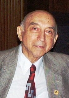
Truth as a matter of degree — but hand-designed, never learned from data.
Not a neural network technique at all, and not a step in the McCulloch-Pitts → Perceptron → backprop chain — a separate, contemporaneous idea. Zadeh's insight: real-world concepts like "warm" or "fast" don't have crisp boundaries, so instead of forcing truth to be strictly 0 or 1, let it be any value in between — 0.7 "true," representing a degree of membership rather than a hard yes/no.
A fuzzy system is built from human-written rules ("IF temperature is warm AND humidity is high THEN fan
speed is medium-high") using hand-designed membership functions — there's no training loop, no
loss.backward(), no learning from examples at all. It became a genuine commercial success
story in the late 1980s–90s, especially in Japan, showing up in washing machines, camera autofocus, subway
train controllers, and air conditioners — maturing at almost exactly the same moment neural networks were
just recovering from the AI winter via backpropagation.
Despite the "digital vs. analog" framing being tempting, fuzzy logic is almost always run as ordinary floating-point software on ordinary digital computers — it's a digital simulation of a continuous-valued idea, not literal analog hardware. (Ironically, it's modern neural networks' smooth activation functions that map most directly onto real analog computing chip research today.)
📄 Fuzzy Sets (1965), Information and Control
1969 — Minsky & Papert's Perceptrons
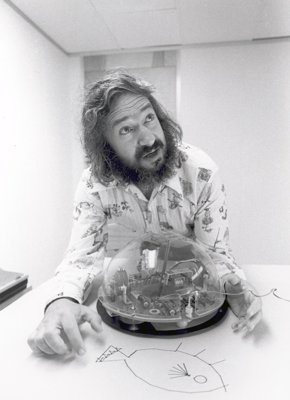
A rigorous proof of the single-neuron ceiling — and the start of the "AI winter."
Minsky and Papert mathematically proved what the 1943 model already hinted at: a single-layer perceptron can never solve XOR, or anything else that isn't linearly separable. They acknowledged that stacking multiple neurons into layers could in principle overcome this — but were openly pessimistic anyone would find a way to actually train such a stack. That pessimism, more than the limitation itself, is widely credited with gutting funding and interest in neural network research for over a decade.
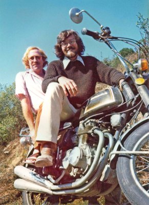
1965–1972 — Hubert Dreyfus: "What Computers Can't Do" philosophical throughline
Berkeley philosopher's direct, sustained attack on symbolic AI — arriving years before the field itself recognized the problem.
Dreyfus's 1965 RAND paper "Alchemy and Artificial Intelligence" and 1972 book What Computers Can't Do (revised in 1992 as What Computers Still Can't Do) drew on Heidegger and Merleau-Ponty's phenomenology to attack the core assumption of "GOFAI" (Good Old-Fashioned AI) — that intelligence is fundamentally symbol manipulation according to explicit rules. His argument: human expertise is tacit, embodied, holistic, and contextual, not reducible to enumerable formal rules — genuine understanding requires being a body, situated in a physical and social world with real needs and stakes, not just processing symbols.
The AI community's reaction at the time was hostile, sometimes personally so. But his specific target — GOFAI — is exactly the Expert Systems paradigm in the very next entry below, and it collapsed for almost exactly the reasons he named: brittle, no genuine common sense, unable to handle context outside narrow hand-coded rules (what he and others called "the frame problem"). Notably, Dreyfus was not simply anti-AI — he held guarded optimism toward connectionist/neural-network approaches specifically because they're sub-symbolic and pattern-based, much closer to his own account of tacit understanding.
Late 1970s–80s — Expert Systems what "mainstream AI" actually was during the neural-network dark ages
A huge commercial boom, then a bust — and the real answer to "surely something happened in that gap."
While neural networks sat in the funding wilderness after Minsky & Papert, a completely different, non-neural approach dominated AI research and industry: expert systems — programs that encoded a human expert's knowledge as explicit IF-THEN rules, plus an "inference engine" that chained rules together to reach conclusions. MYCIN (Stanford, diagnosing bacterial infections) and XCON/R1 (Digital Equipment Corporation, configuring complex computer orders) were the famous examples — XCON reportedly saved DEC on the order of $40 million a year by the mid-1980s. This was a genuine, large-scale commercial AI boom, complete with dedicated LISP-machine hardware companies.
It collapsed starting around 1987 — hence "Expert Systems" being the actual majority of AI funding and attention during exactly the years neural networks were dormant. Every new rule had to be manually extracted from a human expert (slow, expensive "knowledge engineering"), the systems were completely brittle outside their narrow hand-coded domain, and the specialized LISP-machine companies got wiped out once cheaper general-purpose workstations became powerful enough. This collapse is specifically called the second AI winter.
1986 — Rumelhart, Hinton & Williams: Backpropagation
How to actually train a hidden layer — the fix that ended the winter.
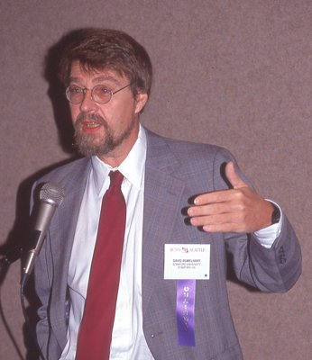
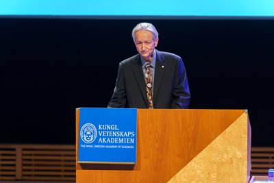
The hard problem wasn't "use 2 neurons instead of 1" — it was figuring out how to assign credit/blame to a hidden-layer neuron's weights when you only know if the final output was right or wrong. This 1986 Nature paper demonstrated the fix: backpropagation, using calculus (the chain rule) to push the output error backward through every layer. It's the same algorithm — completely unchanged in its core math — behind every model we've trained on this site, including the tiny GPT-2 and the network below.
Here's a 2-hidden-neuron network, trained live via this exact algorithm, finally solving XOR:
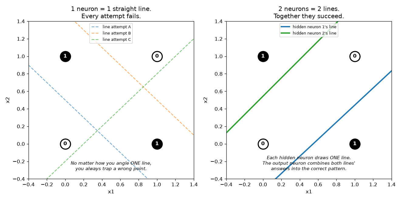
Any single straight line (left, dashed attempts) always traps a wrong point — mathematically impossible to avoid, since XOR's 1s and 0s sit on opposite diagonal corners. Two lines together (right) succeed.
Now the same network, drawn the EE way — two summing-junction/comparator neurons (h1, h2), each with its own real learned weights and boundary line, feeding a third comparator neuron that combines their two yes/no answers into the correct XOR result:
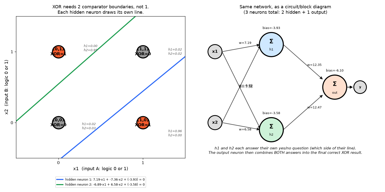
Each hidden neuron only ever answers one question — which side of its own line. Neither answer alone tells you XOR's correct output; only the output neuron's combination of both does. That combination step is exactly what a single neuron structurally cannot do.
📄 Learning representations by back-propagating errors (1986), Nature
1989 & 1998 — Yann LeCun: Convolutional Neural Networks (LeNet)
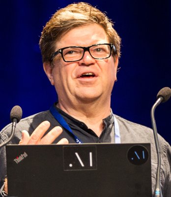
Same Yann LeCun who shows up later in this page's critiques section (2022, arguing pure LLMs are a dead end) — decades earlier, he was the one who made images practical for neural networks at all.
Every network on this page so far has been fully connected — every input wired to every neuron with its own independent weight (our XOR net, the perceptron). For an image, that's a real problem: a modest 200×200 pixel image has 40,000 inputs, and a fully-connected hidden layer would need a separate weight for every input-to-neuron connection — millions of weights before you've done anything useful, and no way to reuse what's learned about detecting an edge in one part of the image when that same edge shows up somewhere else.
LeCun's fix, applied practically in 1989 (reading handwritten ZIP codes for the US Postal Service at Bell Labs) and refined into the famous 7-layer LeNet-5 in 1998: a small filter — a tiny grid of shared weights, far smaller than the image itself — slides across the entire image, computing the same weighted sum at every position. The same 9 numbers detect a vertical edge whether it appears in the top-left corner or dead center — one filter, reused everywhere, instead of a separate weight for every pixel position. This is convolution, and it's the "C" in CNN.
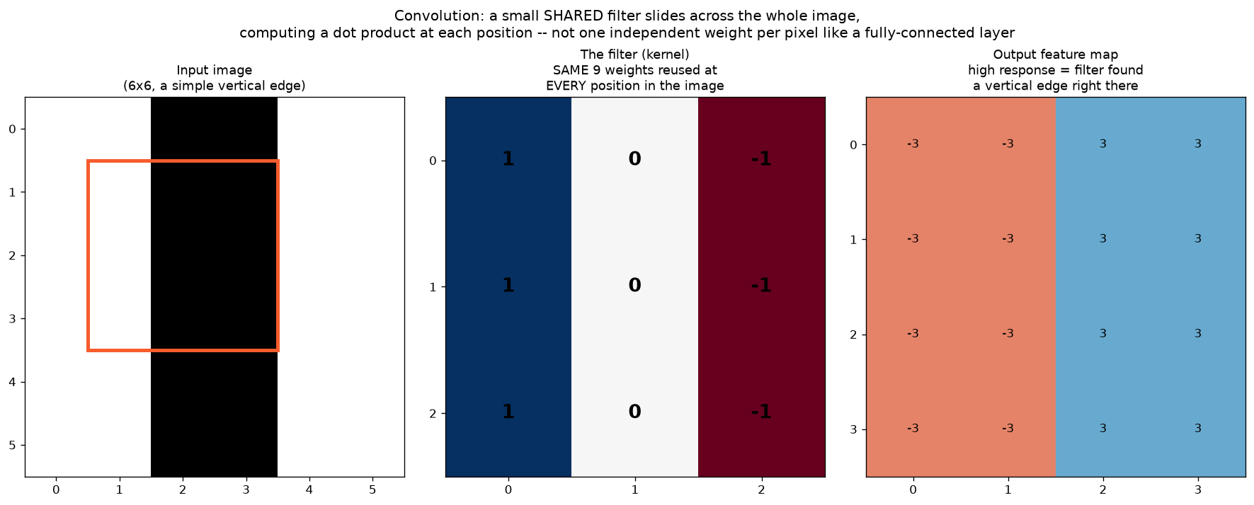
Stack several of these convolution layers (each followed by "pooling" — downsampling that keeps only the strongest response in each small region) and something powerful happens: early layers learn to detect simple local features like edges, exactly like the filter above; deeper layers combine those into progressively more complex shapes, textures, and eventually whole objects. LeNet-5 had about 60,000 parameters total — tiny by today's standards, but it's the direct architectural ancestor of the network in the very next entry.
1990 — Jeffrey Elman: The "Vanilla" Recurrent Neural Network
The first network on this page with a genuine memory — and the direct ancestor of the RNN/LSTM lineage.
Everything up to this point (perceptron, XOR net) has been feedforward: data goes in, flows straight through once, comes out — no memory of anything that came before. That's fine for a fixed input like two logic signals, but useless for a sequence (a sentence, read one word at a time), where what came earlier genuinely matters for what comes next.
The "recurrent" idea has an older, more tangled history than one clean date: the Hopfield Network (1982) was the first well-known network with feedback loops, though it's structured differently enough that it's not always counted as part of the same family; the Jordan Network (1986) first defined "recurrent" the way we mean it here (output feeding back into the hidden layer). Elman's 1990 network is the one usually meant by "plain RNN" today, and the first successfully trained with backpropagation.
The internal structure: at each time step, a single "cell" takes two things as input — the current word/token, and its own hidden state carried over from the previous step — and produces an output plus an updated hidden state that gets passed to the next step. That hidden state is the network's only memory of everything it's seen so far, compressed into one vector.
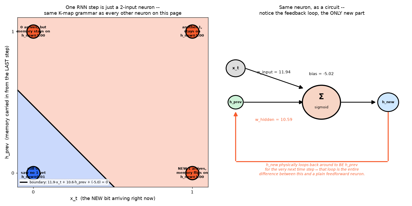
Reading this in the same K-map style as every neuron so far: at any single time step,
an RNN cell is just a 2-input neuron — its two inputs are the new incoming value (x_t)
and the memory carried in from the last step (h_prev), combined by a weighted sum + sigmoid,
exactly like the perceptron. The only genuinely new ingredient is the loop on the right: the output
(h_new) gets physically routed back around to become h_prev for the next step.
These are the real learned weights from actually training a minimal 1-hidden-unit RNN on a "remember if a
1 has ever appeared" task:
1997 — LSTMs: Solving Memory for Sequences
Backprop could now train hidden layers, but plain recurrent networks still "forgot" anything more than a few steps back.
Hochreiter & Schmidhuber's Long Short-Term Memory network addressed the specific problem the previous entry's ⚠️ box named: once you chain many small steps together (like reading a sentence word by word), the gradient signal from backprop tends to shrink to nothing (or explode) as it's pushed back through many steps — the "vanishing/exploding gradient" problem. LSTMs added explicit "gates" (learned mechanisms deciding what to keep, forget, or output at each step) that let a network carry information across many more steps reliably, without changing the basic recurrent shape from the entry above.
This became the dominant way to handle language, speech, and any sequential data for the next two decades — right up until the 2017 entry below replaced it.
Now zooming out to see many of these steps chained together over time, and how that compares to a Transformer processing the whole sequence at once instead:
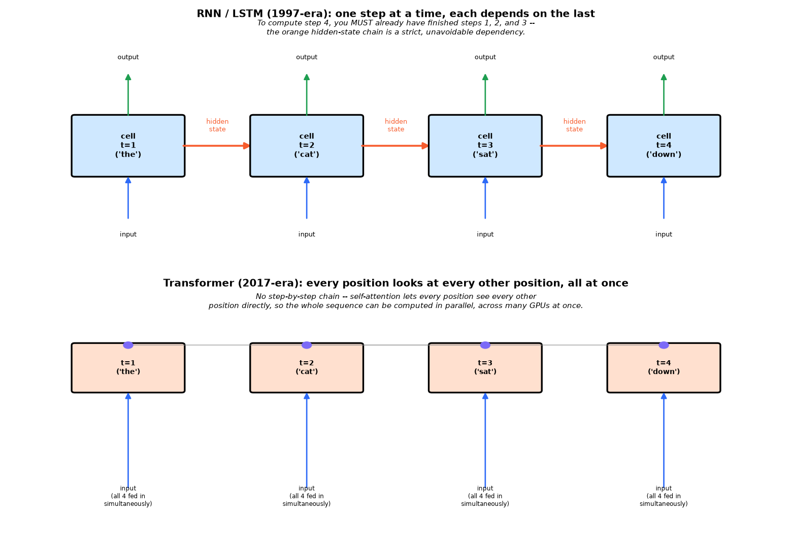
Look at the top half of the diagram: computing step 4 strictly requires steps 1, 2, and 3 to already be finished — that orange hidden-state chain cannot be skipped or reordered. This is exactly the "strictly sequential" limitation the ⚠️ box below describes, and it's the direct reason the 2017 entry replaced this architecture rather than just scaling it up further.
📄 Long Short-Term Memory (1997), Neural Computation
1999–ongoing — Ray Kurzweil: The Optimist's Case the counter-argument to everything above
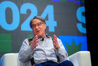
Every critique above assumes AI has real limits worth naming. Kurzweil's entire career is betting the limits are temporary.
Kurzweil's 1999 prediction — human-level AI (AGI) by 2029, and "the Singularity" (AI recursively self-improving beyond combined human intelligence, and merging with humans) by 2045 — long predates this entire LLM era, and he has not moved the date despite 25+ years passing, reaffirming 2029 in his 2024 book The Singularity Is Nearer. His argument rests on "the Law of Accelerating Returns" — information technologies improve exponentially, and exponential curves look deceptively flat right up until they don't.
His track record is genuinely contested, not simply good or bad: Kurzweil claims 86% accuracy on his own past predictions, and cites real, specific hits (smartphones, cloud computing, both predicted with real precision years in advance). But an independent 2019 assessment (Stuart Armstrong, Future of Humanity Institute) found only 42% accuracy — less than half his self-reported figure — largely because many predictions are vague enough to grade generously, or have timelines that quietly shift.
2012 — AlexNet and the ImageNet Moment
Backprop was 26 years old by now — what actually changed was data and compute, not the algorithm.
Alex Krizhevsky, Ilya Sutskever, and Geoffrey Hinton (yes — the same Hinton from the 1986 paper) trained a deep convolutional neural network on consumer GPUs and entered the ImageNet competition — 1000 object categories, 1+ million labeled training photos. It won by a shocking margin, roughly halving the error rate of the best non-neural-network approach in a single year. This is widely regarded as the moment that convinced the broader field deep neural networks, given enough data and compute, could dramatically outperform every hand-engineered alternative.
Why 2012, and not 1986? The algorithm hadn't changed — backpropagation is the same algorithm we ran ourselves. Two other ingredients finally caught up: enough labeled data existed (ImageNet itself, a massive human-labeled dataset assembled over the preceding years), and enough cheap, parallel compute existed — consumer GPUs, originally built for video game graphics, turned out to be extraordinarily well-suited to the matrix multiplications neural networks need. This is the exact "scaling" story from our earlier conversation this session, playing out for the first time.
📄 ImageNet Classification with Deep Convolutional Neural Networks (2012), NeurIPS
2014 — Ian Goodfellow: Generative Adversarial Networks (GANs)
Two networks locked in competition with each other — the dominant way to generate realistic images for the better part of a decade, before diffusion models took over.
Goodfellow's idea, reportedly worked out during a late-night discussion with friends in 2014: train two neural networks against each other in a zero-sum game. A generator network tries to produce fake images realistic enough to fool a second network; a discriminator network tries to correctly tell real images (from a training set) apart from the generator's fakes. Both networks improve together — as the discriminator gets better at spotting fakes, the generator is forced to get better at fooling it, and vice versa — a self-sustaining competitive loop rather than a single network learning from a fixed, direct target the way everything else on this page has so far.
2015 — Sohl-Dickstein et al.: Diffusion Models, the Theory
A genuinely different generative idea, borrowed directly from statistical physics — years before it was practical enough to matter.
"Deep Unsupervised Learning using Nonequilibrium Thermodynamics" proposed a different generative strategy entirely: instead of two networks competing (GANs), take real training images and gradually destroy them by mixing in more and more random noise, step by step, until nothing recognizable remains — this "forward process" needs no learning at all, it's just a fixed noising recipe. Then train a single neural network to do the reverse: given a noisier image, predict a slightly less noisy version of it. Chain that reverse step many times, starting from pure random noise, and — if it works — a realistic image gradually emerges.
This 2015 paper was purely theoretical grounding, explicitly inspired by non-equilibrium thermodynamics in physics — it did not yet produce results competitive with GANs, and the idea sat relatively unnoticed for five years until the next entry made it actually practical.
2017 — "Attention Is All You Need": The Transformer
Removed the strict step-by-step requirement entirely — the architecture behind every frontier model since, including the one you're talking to.
A team at Google introduced the Transformer, built around "self-attention" — instead of processing a sequence one step at a time carrying a hidden memory forward (the LSTM way), every position in the sequence looks directly at every other position simultaneously, weighing how relevant each one is to each other. This removed LSTMs' core bottleneck: since there's no step-by-step dependency, an entire sequence can be processed in parallel across many GPUs at once.
This is the exact architecture family behind the tiny GPT-2 we downloaded, trained, and ran earlier — and behind every current frontier model (GPT, Claude, Gemini, Llama). "Decoder-only causal transformer," the term from our very first conversation on this topic, refers to a specific way of using this 2017 architecture for next-token text generation.
Inside one block — this is the repeating unit that gets stacked N times (5 in our tiny demo, 96 in GPT-3, per the scale comparison above). Tokens get embedded into vectors, self-attention lets every position gather information from every other position at once, then a small feed-forward network (an ordinary MLP, the same building block from every network we've trained this session) processes each position — with "Add & Normalize" residual connections stabilizing training as this stacks very deep:
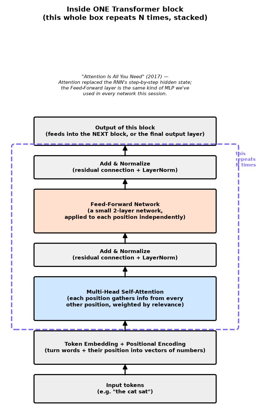
Forward propagation here is exactly the same concept as our XOR worked example above, just with far
more (and more complex) steps in between input and output — data flows up through this diagram, a real
number at every stage. Backward propagation is the same chain rule too, just automatically differentiating
through attention and the feed-forward layers instead of through two summing-junction neurons — the same
loss.backward() call, just walking back through a much longer chain.
📄 Attention Is All You Need (2017), arXiv
2018–ongoing — Gary Marcus: The Sustained Skeptic philosophical throughline
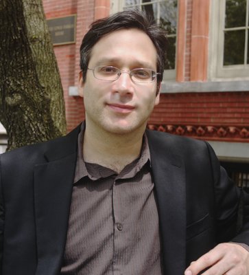
Cognitive scientist arguing, since before the current LLM boom, that pure deep learning needs to be paired with symbolic reasoning, not replace it.
Marcus's 2018 paper "Deep Learning: A Critical Appraisal" and 2019 book Rebooting AI (with Ernest Davis) predate ChatGPT by years, arguing that pure neural-network pattern-matching — no matter how large — would keep failing at tasks requiring genuine compositional reasoning, reliable factual grounding, and common sense, and that hybrid neuro-symbolic systems (combining learned pattern recognition with explicit symbolic reasoning) were necessary. He has remained a constant, high-visibility critic through the entire LLM era, frequently cataloguing specific failure cases (hallucinations, reasoning errors, brittleness on novel compositions) as evidence the underlying limitation hasn't actually gone away, just gotten harder to spot.
2018–2020 — GPT-1, GPT-2, GPT-3: The Scaling Era Begins
Same architecture as 2017, mostly just made bigger and bigger — and it kept working.
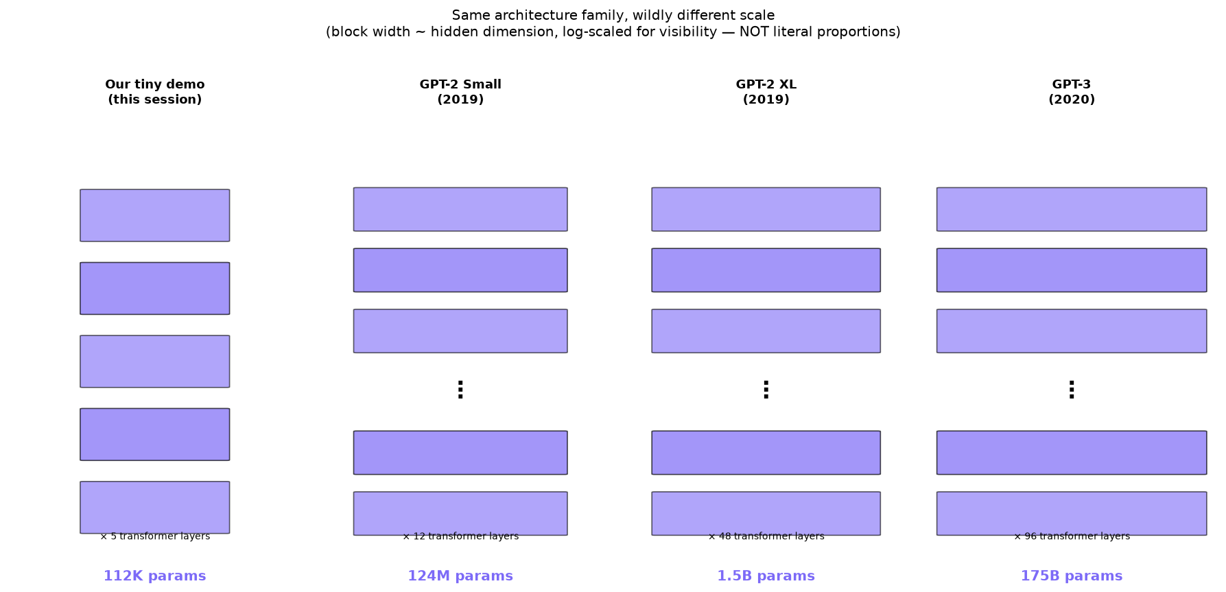
OpenAI applied the 2017 Transformer architecture specifically to the task of predicting the next word in huge amounts of text, at increasing scale: GPT-1 (2018, 117M parameters) proved the approach worked at all; GPT-2 (2019, up to 1.5B parameters — the same architecture as our tiny demo, just ~13,000x bigger) was notable enough that OpenAI initially withheld the full model over misuse concerns; GPT-3 (2020, 175B parameters) demonstrated "few-shot learning" — performing new tasks from just a handful of examples in the prompt, with no retraining at all.
Alongside GPT-3, OpenAI published empirical scaling laws (Kaplan et al., 2020) showing model performance improved smoothly and predictably as parameters, data, and compute all increased together — the empirical backbone of the entire "just make it bigger" era, and the same scaling-laws conversation we had earlier this session.
What "bigger" actually looks like — same architecture family throughout (the 2017 Transformer), just stacked deeper and wider each generation. Not drawn to scale or with every connection shown, just the shape (number of layers stacked) and the real parameter counts:
📄 Language Models are Few-Shot Learners (GPT-3, 2020), arXiv
2020 — Lewis et al.: Retrieval-Augmented Generation (RAG)
A direct answer to the "stochastic parrot"/hallucination problem — let the model look things up instead of relying purely on what's baked into its weights.
Lewis et al. (Facebook AI Research, University College London, and NYU), presented at NeurIPS 2020, proposed combining two different kinds of "memory": a language model's own parametric memory (whatever got baked into its weights during pretraining — everything covered in the entry above) with an external non-parametric memory — a real, searchable document collection the model can query at answer time. The mechanism has two parts: a retriever searches that document collection (typically using embedding-based similarity search) for passages relevant to the current question, and a generator (the language model itself) is given both the question and those retrieved passages as context, producing an answer actually grounded in real, specific source text rather than purely from statistical patterns memorized during training.
This directly addresses a concern from the Stochastic Parrots entry below: a model that can retrieve and cite real documents is at least partially checkable and groundable, rather than purely confabulating fluent-sounding text from training statistics. It also solves a separate, practical problem pretraining alone can't: giving a model access to information that's newer than its training cutoff, or specific to a private document collection, without needing to retrain the whole model.
2020 — Ho, Jain & Abbeel: DDPM Makes Diffusion Actually Work
The paper that turned 2015's theory into genuinely competitive image quality — the direct ancestor of every major image generator since.
"Denoising Diffusion Probabilistic Models" (UC Berkeley) refined Sohl-Dickstein's 2015 framework with specific, practical training choices that made the resulting image quality genuinely competitive with — and soon better than — GANs. Same core idea as 2015 (fixed forward noising, learned reverse denoising, illustrated below with our own tiny synthetic image), but with the specific mathematical and architectural refinements that made it actually work well in practice for the first time.
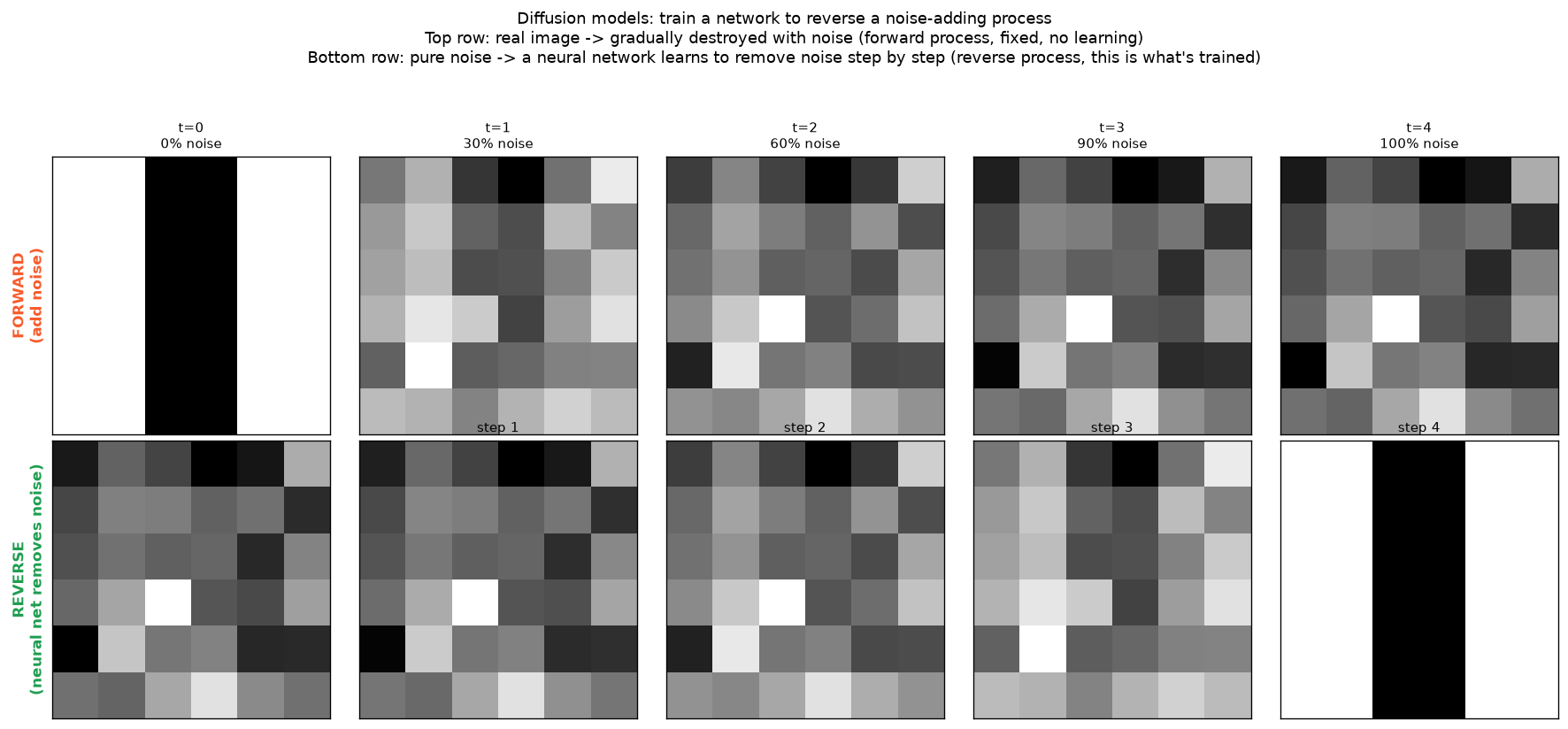
Honest note on the diagram above: the reverse row shown here just replays the same fixed noise sequence backward, to illustrate the concept clearly — a real trained diffusion model's reverse process is a genuinely learned neural network prediction at each step, not a simple replay, and actually training one from scratch is a much larger undertaking than the small demos elsewhere on this page.
2021 — "On the Dangers of Stochastic Parrots" philosophical throughline
The paper that coined the exact phrase used throughout this whole page's discussion of whether LLMs "understand" anything.
Bender, Timnit Gebru, and co-authors' 2021 paper argued large language models are sophisticated statistical pattern-matchers over text — "stochastic parrots" — fluently reproducing the form of language without any grounding in meaning, reference, or communicative intent. The paper's concerns went beyond philosophy: it raised the environmental cost of training ever-larger models, the risk of baking in and amplifying bias present in scraped training data, and the danger of fluent output creating an illusion of understanding that could mislead users and researchers alike.
This is the direct academic source of the "stochastic parrots" framing referenced repeatedly earlier in this same page's discussion of Dreyfus, embodiment, and whether frontier models "truly" understand anything — not just a casual phrase, but a specific, citable research position with real, ongoing influence on the field.
📄 On the Dangers of Stochastic Parrots (2021), ACM FAccT
2022 — DALL-E 2 & Stable Diffusion: Diffusion Goes Mainstream
The same year as ChatGPT's public moment (next entry) — 2022 was when generative AI broadly, not just text, reached the public all at once.
OpenAI's DALL-E 2 (April 2022) combined a diffusion model with CLIP (a separate model trained to understand the relationship between images and text captions), letting a written prompt guide the reverse denoising process toward an image matching that description — the key ingredient that makes "type a sentence, get a picture" possible at all. Stable Diffusion (Stability AI, LMU Munich, and RunwayML, August 2022) used the same underlying diffusion approach but was released publicly and openly — the model weights themselves, not just an API — making high-quality text-to-image generation runnable on a consumer GPU for the first time, a genuinely different accessibility choice from DALL-E 2's closed, hosted-only approach.
2022 — ChatGPT: The Public Moment
Not a new architecture — a product/interface moment that made this whole lineage visible to the world.
ChatGPT wrapped an already-existing GPT-3-family model in a simple chat interface and made it free and public. Nothing about the underlying 2017-architecture technology was new — what changed was accessibility. It became one of the fastest-adopted consumer products in history, and is the moment "AI" (specifically, this decoder-only-transformer lineage) went from a research/enterprise topic to mainstream public awareness — directly setting the stage for the investment, hype, and scrutiny (including the DeepSeek distillation disputes) we discussed earlier this session.
2022–ongoing — Yann LeCun: "Autoregressive LLMs Are a Dead End" philosophical throughline, still unresolved
A living, current critique from deep inside the field itself, not yet a settled historical verdict like Dreyfus.
LeCun (Turing Award winner, former Meta Chief AI Scientist) has argued publicly since 2022 that autoregressive LLMs — predicting one token at a time, exactly the mechanism behind our own tiny GPT-2 and every model in the 2018–2020 entry above — are fundamentally limited: small errors compound token by token, and the architecture has no genuine model of the physical world, so it "can't truly reason or plan" or predict the consequences of actions. His alternative, JEPA (Joint Embedding Predictive Architecture), predicts outcomes in a compressed, abstract representation space instead of generating output token by token — closer, in his view, to how a brain runs a fast mental simulation rather than imagining every physical detail.
Unlike Dreyfus, this critique is unresolved in real time — LeCun has continued pursuing this direction independently, and whether JEPA-style world models overtake pure autoregressive scaling, get absorbed as one component of hybrid systems, or turn out to be unnecessary is a genuinely open question this page cannot yet give a historical verdict on.
2023 — Noam Chomsky: "The False Promise of ChatGPT" philosophical throughline
A linguistic critique, distinct from Dreyfus's phenomenology or LeCun's world-models argument.
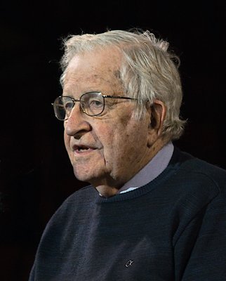
Chomsky and co-authors' 2023 New York Times op-ed argued LLMs are categorically different from, and inferior to, genuine human language ability. His decades of linguistic theory hold that human language reflects an innate, universal grammar — a genuine generative system capable of understanding deep structure, causation, and what is impossible as well as what's likely. LLMs, by contrast, are statistical engines fitting patterns in existing text — capable of describing what usually happens, not explaining why, and just as able to learn "possible" and "impossible" human languages equally well, which he takes as proof they aren't modeling anything like real linguistic competence at all.
2024–2025 — Reasoning Models & Test-Time Compute (o1/o3)
The second scaling axis — already discussed this session, formally added here now.
As pure pretraining scale (bigger models, more data) started showing diminishing returns, OpenAI's o1 (and successor o3) introduced a different lever: instead of answering immediately, the model generates an extended internal chain of reasoning steps before producing a final answer, using reinforcement learning during training to learn to reason well, then spending more compute per question at the moment you actually ask it something — "thinking longer" on harder problems.
2024 — Anthropic: The Model Context Protocol (MCP)
Not a model or a training technique — a standardized plug for connecting AI to tools and data, and literally what's running underneath this very conversation.
Anthropic open-sourced MCP on November 25, 2024: an open standard for how an AI assistant connects to external tools, data sources, and services — Google Drive, GitHub, a database, a trading platform, anything — without every single AI application needing its own bespoke, one-off integration code for every tool it wants to use. An "MCP server" wraps access to one specific tool or data source in a consistent, discoverable format; any MCP-compatible AI client (like Claude Code, running this session) can then connect to any MCP server and use its capabilities the same standardized way.
This is directly, concretely running right now, not an abstract example: the EDGAR filings lookup, the Robinhood trading tools, and the sentiment-analysis tools available in this very environment are real MCP servers — and everything on this page was built by an MCP client (this conversation) calling them.
Adoption was unusually fast and unusually cross-company for a standard originated by one AI lab: OpenAI adopted MCP across its own products by March 2025, Google DeepMind added support in Gemini by April 2025, and Microsoft/GitHub joined its steering committee by May 2025. In December 2025, Anthropic donated MCP to the Agentic AI Foundation, a Linux Foundation project co-founded with Block and OpenAI — turning a single-company standard into genuinely neutral, shared infrastructure.
Full text timeline now complete through today — next pass: go back through and discuss/fix each entry in depth, plus add per-entry diagrams where useful.
👥 Who's Building This: Key Researchers Today
Not a ranking — a working roster of the people whose names show up most across current frontier AI, and what they specifically contributed.
The Transformer authors — Google Brain, 2017
Worth stating plainly: the architecture behind every current frontier model, including the one you're talking to, came out of Google — not OpenAI, not DeepMind.
Vaswani, Shazeer, and five co-authors (Jakob Uszkoreit, Illia Polosukhin, Aidan Gomez, Łukasz Kaiser, Niki Parmar) wrote "Attention Is All You Need" at Google Brain in 2017 — already the subject of its own entry earlier on this page. Shazeer specifically later left to co-found Character.AI, then returned to Google in 2024 — a good example of how fluidly researchers move between these companies.
Dario Amodei — Anthropic

Co-authored the actual scaling-laws paper already referenced in the 2018–2020 GPT entry above, before founding the company that builds the model answering these questions right now.
Amodei was a co-author on GPT-2 and GPT-3 at OpenAI, and on the Kaplan et al. scaling-laws paper — the empirical backbone of the "just make it bigger" era already covered on this page. He left OpenAI in 2021 to found Anthropic, with a safety-focused research agenda as the founding motivation.
Demis Hassabis — Google DeepMind
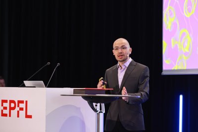
Co-founded DeepMind, acquired by Google in 2014 — now "Google DeepMind."
Led AlphaGo (2016, beat the world Go champion using reinforcement learning + tree search, a genuinely different technique family from anything on this page's neural-network timeline) and AlphaFold (protein structure prediction) — the latter won him the 2024 Nobel Prize in Chemistry, awarded the same year Hinton won the Physics prize for backpropagation-adjacent work.
Fei-Fei Li — Stanford
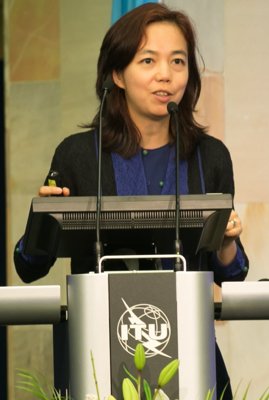
Built the dataset, not the model — but without it, the 2012 AlexNet entry on this page doesn't happen.
Li led the creation of ImageNet — the massive, human-labeled image dataset (1000 categories, 1M+ images) that AlexNet was trained and evaluated on. A direct, concrete reminder that the "scaling" story on this page isn't just about bigger models — it needed bigger, well-labeled datasets just as much.
Andrej Karpathy — educator and practitioner
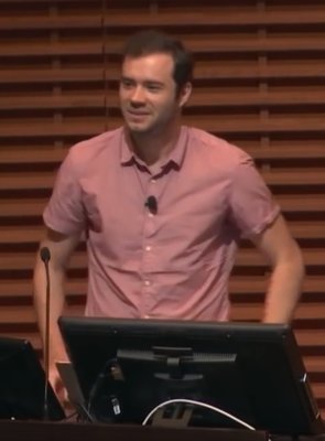
Former Tesla Autopilot lead and OpenAI founding member, now best known for making exactly this kind of from-scratch, verified, no-magic teaching material.
His minGPT/nanoGPT projects — small, fully transparent, from-scratch GPT implementations anyone can read top to bottom — are close in spirit to this whole page's own approach: build the tiny real version yourself rather than take the architecture on faith.
Jeff Dean — Google Chief Scientist
Built the infrastructure the rest of this section runs on, more than any specific model.
Co-created TensorFlow and led Google's large-scale distributed training systems — the software plumbing that makes training models at the scale described in this page's "model scale comparison" section physically possible in practice, not just on paper.
Already covered elsewhere on this page
Geoffrey Hinton, Ilya Sutskever, and Yann LeCun all appear in full earlier — Hinton and Sutskever in the 1986 Backprop and 2012 AlexNet entries, LeCun in the critiques section above (2022–ongoing, JEPA/world models) — rather than repeating them here.
🔬 Concept Deep-Dives
Not part of the chronological timeline above — standalone explainers for specific mechanics that come up repeatedly.
📋 Cheat Sheet / Glossary
Every term used across this page, in one place — vocabulary accumulates fast over a multi-day project.
Building Blocks
- Neuron
- The basic unit: multiply each input by a weight, sum them plus a bias, then pass the result through an activation function.
- Weight
- A number multiplying one input — how much that input matters to this neuron. Learned from data (1958 onward), not hand-picked (1943).
- Bias
- A constant added to the weighted sum, independent of any input — shifts the decision boundary off the origin. See the 1958 entry for why this matters.
- Activation function
- What turns the weighted sum into the neuron's output — step (hard on/off), sigmoid, ReLU, or GELU. See the Activation Functions deep-dive.
- Threshold / comparator
- EE framing of activation: a neuron firing at
sum ≥ 0is exactly a comparator firing at a reference voltage.
Architectures
- Perceptron
- Rosenblatt's 1958 single trainable neuron. One neuron, no hidden layer — a "network" of size one.
- Hidden layer
- Any layer of neurons between input and output. "Hidden" means not part of the input/output interface — not unobservable; we can and do inspect it directly.
- Multi-Layer Perceptron (MLP) / feedforward network
- Neurons arranged in layers, data flows straight through once (no loops). Our XOR network is the simplest real example.
- Feedforward
- Data moves one direction only, input toward output, no feedback loops — as opposed to recurrent.
- RNN (Recurrent Neural Network)
- Processes a sequence one step at a time, feeding its own previous output/hidden-state back in as memory. Not the same word as "Recursive" Neural Network (a different, rarer, tree-structured architecture). We have not built an RNN this session — only diagrammed one for comparison.
- LSTM (Long Short-Term Memory)
- A specific gated RNN design (Hochreiter & Schmidhuber, 1997) that fixes plain RNNs' vanishing-gradient problem over long sequences.
- Transformer
- The 2017 architecture ("Attention Is All You Need") behind every current frontier model. Processes all sequence positions in parallel via self-attention, instead of RNN's one-step-at-a-time approach.
- Self-attention
- The mechanism inside a Transformer where every position looks at every other position at once, weighing relevance, instead of relying on a passed-along hidden state.
Training
- Supervised learning
- Training data includes the correct answer for every example (what all our demos this session have used). Unsupervised = no correct answers given, algorithm finds structure on its own.
- Loss function
- A number measuring how wrong the current output is versus the correct answer — what training tries to minimize.
- Gradient descent
- Adjusting parameters in the direction that reduces the loss, using the loss function's derivative (gradient).
- Backpropagation ("backprop")
- The 1986 algorithm for computing that gradient for every weight in a multi-layer network, via the chain rule, working backward from the output.
- Chain rule
- The calculus rule that lets you multiply local derivatives together across layers to get a gradient for an early weight — see the worked XOR example above.
- Learning rate
- How big a step each weight update takes. Too small = slow; too large = coarse/unstable (in gradient-descent methods — the plain perceptron rule is more forgiving, per the Perceptron Convergence Theorem).
- Epoch
- One full pass through the entire training dataset.
- Linearly separable
- A problem solvable by a single straight-line (or hyperplane) boundary. AND/OR are; XOR/XNOR are not — the core reason multi-layer networks are needed at all.
Scale & Modern Practice
- Parameters
- The total count of learned weights + biases in a model. Our tiny demo: 112K. GPT-3: 175B.
- Scaling laws
- Empirical finding (Kaplan et al., 2020) that performance improves smoothly and predictably as parameters/data/compute all grow together.
- Fine-tuning / SFT (supervised fine-tuning)
- Further training an already-pretrained model on human-written example responses, to align its behavior.
- RLHF
- Reinforcement Learning from Human Feedback — trains a separate reward model on human preferences, then uses RL (typically PPO) to optimize the model against it. See the "RLHF and DPO" deep-dive below for the full pipeline.
- DPO
- Direct Preference Optimization — mathematically collapses RLHF's two stages (reward model + RL) into one direct optimization on preference data, no separate reward model or RL loop needed.
- Reasoning models / test-time compute
- o1/o3-style models (2024–2025) that spend extra compute "thinking" via an internal chain of steps before answering, rather than answering instantly.
Software / Hardware Pipeline
- Compiler
- Translates source code into assembly (and eventually machine code). Heuristic-based, not perfect — see the gcc
-O0vs-O2comparison. - Assembly
- Human-readable mnemonics for CPU instructions, one step above raw machine code bytes.
- Machine code
- The actual bytes the CPU executes — e.g.
01 d0for our adder'sadd eax, edx. - Object file (
.o) - Compiled machine code plus a manifest of what it defines/needs — not yet a runnable program.
- Linker
- Combines object files, resolving each undefined symbol to a real final address, producing one runnable executable.
- Interpreted language
- Executed by another program (an interpreter) reading it step-by-step at runtime, rather than compiled fully to native machine code ahead of time. Python via CPython is interpreted; C is compiled.
- JIT (Just-In-Time compilation)
- Compiling hot code paths to real machine code at runtime, after observing they're actually used a lot — see the Numba demo.
Architecture Shapes, Side by Side
Feedforward, Recurrent, Transformer, Recursive, CNN, GAN, Diffusion — same basic ingredient (neurons + weights), seven very different connection patterns.
Not to scale, and not every connection drawn — just the structural shape of how data flows through each one:
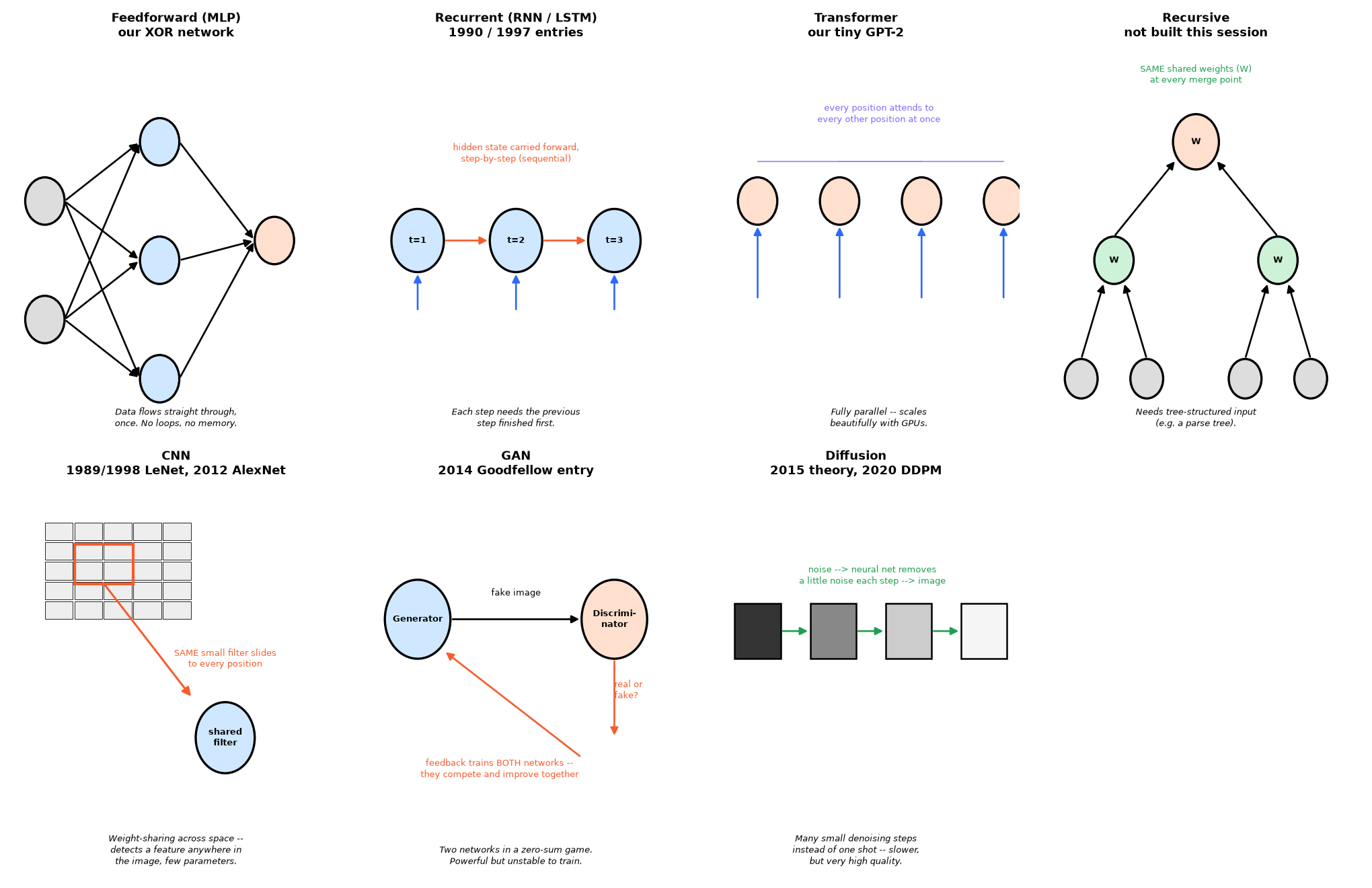
| Architecture | Data flow | Good at | Bad at | Real examples |
|---|---|---|---|---|
| Feedforward (MLP) | Straight through, once. No loops, no memory of previous inputs. | Fixed-size inputs with no inherent order/sequence — tabular data, simple classification. Fast, simple, easy to train. | Anything with sequence or variable length (text, audio, time series) — has no way to use position/order information at all. | Our XOR/OR-gate networks; the feed-forward sub-layer inside every Transformer block. |
| Recurrent (RNN / LSTM) | One step at a time, carrying a hidden-state "memory" forward — each step depends on the last. | Sequences where order matters and length varies — was the standard for language/speech/time series for ~20 years. | Strictly sequential — cannot parallelize across a sequence, so training on huge datasets is slow. Long sequences still lose earlier context even with LSTM's fixes. | Pre-2017 machine translation, speech recognition, older predictive-text keyboards. |
| Transformer | Every position attends to every other position simultaneously — fully parallel, no step-by-step dependency. | Sequences at massive scale — parallelizes perfectly across many GPUs, captures long-range relationships directly. | Attention cost grows quadratically with sequence length — very long inputs get expensive. Needs lots of data/compute to train well from scratch. | GPT, Claude, Gemini, Llama — every current frontier language model, plus our own tiny GPT-2 demo. |
| Recursive | The same shared weights applied repeatedly, merging pairs of nodes upward through a tree structure to one root. | Data that's naturally tree-shaped — parsing sentence grammar structure, some program-analysis tasks. | Needs the tree structure to already be known/given — doesn't generalize to plain sequences or unstructured data, so it's a niche choice today. | Historical NLP sentiment/parsing research (e.g. Stanford's Recursive Neural Tensor Network) — largely superseded by Transformers now. |
| CNN | A small filter of shared weights slides across the whole input, computing the same operation at every position — not one independent weight per input like a fully-connected layer. | Grid-structured data, especially images — detects a learned feature (an edge, a texture) anywhere it appears, with far fewer parameters than a fully-connected layer would need. | Data with no natural grid/spatial structure — the weight-sharing assumption that makes CNNs efficient for images doesn't help (or apply) for arbitrary tabular or sequence data. | LeNet-5 (1998), AlexNet (2012), most image classifiers; also the feature-extraction backbone inside many diffusion models below. |
| GAN | Two networks in competition: a generator produces fake examples, a discriminator tries to tell real from fake — both improve by trying to beat each other. | Generating sharp, realistic samples quickly — a single forward pass through the generator produces a full image. | Notoriously unstable to train — the two networks can fail to converge together, or the generator can collapse to producing only a narrow range of outputs ("mode collapse"). | Deepfakes, early realistic face generation (StyleGAN), largely displaced by diffusion models for image generation since ~2021. |
| Diffusion | A fixed process gradually adds noise to real data until it's pure static; a neural network is trained to reverse that, removing a little noise at a time across many steps. | High-quality, diverse image (and increasingly video/audio) generation — currently the dominant approach for text-to-image and text-to-video systems. | Slow to generate from — producing one output means running the reverse denoising step many times in sequence, historically much slower than a GAN's single pass (active research area). | DALL-E 2, Stable Diffusion, Midjourney, Sora-style video generation. |
How Alignment Training Actually Works: RLHF and DPO
The step that turns a raw next-word predictor into something that behaves like an assistant — separate from, and after, the pretraining covered in the GPT-era entries above.
A freshly pretrained model (next-token prediction on huge amounts of raw text, fully self-supervised — no human labels involved) has no built-in notion of "helpful," "harmless," or "follow the instruction I actually gave you." Getting from that raw predictor to something that behaves like an assistant takes a further training stage, and there are two different ways the field does it.
RLHF (Reinforcement Learning from Human Feedback) — the original approach, five steps:
1) Start from the pretrained model. 2) Optionally fine-tune it on human-written example responses first (ordinary supervised learning — "supervised fine-tuning," SFT). 3) Instead of paying humans to write full answers (expensive), show them several different model-generated responses to the same prompt and just ask which one is better — ranking is far cheaper than writing. 4) Use that preference data to train a separate reward model — a second neural network whose only job is predicting how a human would rate any given response. 5) Run reinforcement learning (typically an algorithm called PPO) on the original model: generate a response, have the reward model score it, nudge the weights toward whatever scores higher — repeated many times, with no human needed in the loop for each individual step, since the reward model stands in for one.
The honest limitation with RLHF: the reward model is only an approximation of real human preference, and the reinforcement-learning stage can learn to exploit that approximation's blind spots rather than genuinely improve — sounding confident and polished without actually being better. This is called reward hacking, a real, known, unresolved tension in the technique.
DPO (Direct Preference Optimization, Rafailov et al., 2023) — the same goal, one stage instead of two: DPO's actual contribution is a mathematical one — it proves the entire RLHF objective can be solved directly, without ever training a separate reward model or running reinforcement learning at all. Given the same preference data (human picks response A over response B), DPO trains the model directly to raise the probability of the preferred response and lower the probability of the rejected one, using a closed-form loss derived from the same underlying preference math RLHF's reward model was already built on — essentially treating "which one did the human prefer" as a direct classification problem, not something you need an intermediate reward-scoring model and a full RL loop to approach.
What that buys you in practice: no separate reward model to train and maintain, no RL sampling loop, no PPO stability issues to tune around, and less exposure to reward hacking — since there's no separate reward-model proxy sitting in between the preference data and the final model for the optimization to over-fit against.
Activation Functions: Step → Sigmoid → ReLU → GELU
The EE analogy: not a perfect switch, but a transistor's real, soft I-V transition region.
The 1943 neuron used a step function — a hard, instant jump from 0 to 1 at the threshold, exactly like an idealized digital switch. But a real transistor doesn't switch perfectly instantly either — it has a soft "knee," a transition region where it's neither fully off nor fully on. Sigmoid, ReLU, and GELU are different mathematical ways of building that soft transition on purpose.
Sigmoid (which you already know): 1 / (1 + e^-x) — a smooth S-curve,
output always strictly between 0 and 1, approaching but never quite reaching either extreme.
GELU (Gaussian Error Linear Unit — what our tiny GPT-2's config called "gelu_new"):
GELU(x) = x · Φ(x), where Φ(x) is the standard normal (Gaussian) cumulative
distribution function — literally "the probability that a standard normal random variable is less than x."
Intuitively: for a large positive input, Φ(x) ≈ 1, so GELU(x) ≈ x (passes through almost unchanged). For a
large negative input, Φ(x) ≈ 0, so GELU(x) ≈ 0 (mostly zeroed out). Near zero it's smooth and — notably —
dips slightly below zero for small negative inputs, unlike ReLU which clips negatives to exactly 0.
The specific "gelu_new" variant uses a faster tanh-based approximation of Φ(x) rather than computing the
exact Gaussian integral, since tanh is cheaper to compute at the scale of billions of calls.
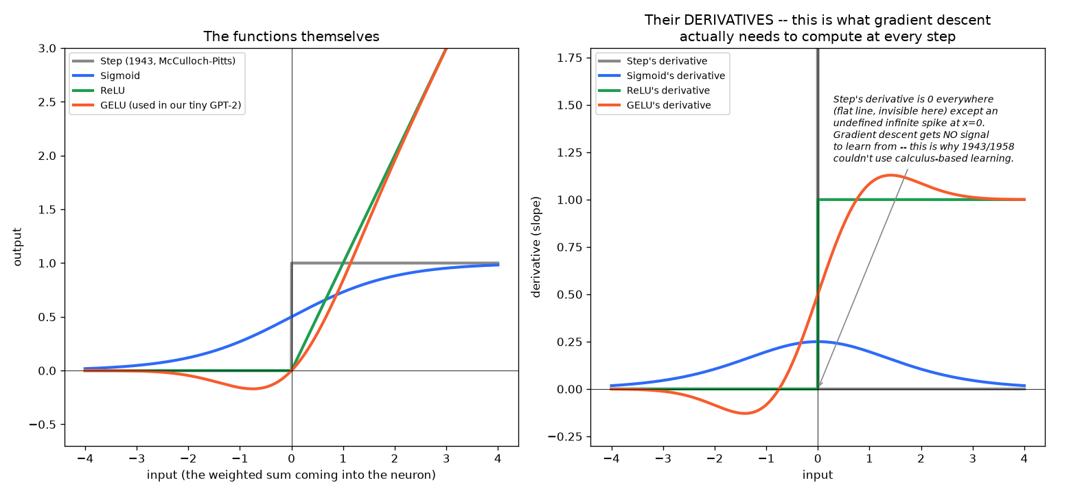
The right panel — the derivatives — is the important one, and it's the direct answer to the next question below: gradient descent needs to know the slope of the activation function at every point to know which direction to nudge a weight. The step function's derivative is 0 everywhere except an undefined infinite spike exactly at the threshold — there's no usable slope anywhere, meaning no gradient signal at all. Sigmoid, ReLU, and GELU all have a real, usable derivative across their whole range, which is precisely why they can be trained by calculus-based methods and a hard step function cannot.
Why did the field move from sigmoid to ReLU, then to GELU? Sigmoid was the natural first choice in 1986 — smooth, and its 0–1 output has a clean "probability-like" feel. But look again at the derivative plot: sigmoid's derivative is a narrow bump, never higher than 0.25, and close to zero once you're away from the center. Stack many layers, and the chain rule multiplies many of these small fractions together — the gradient shrinks toward nothing by the time it reaches early layers. This is the vanishing gradient problem, and it made genuinely deep networks (many layers) impractical to train for years.
ReLU (used heavily starting with AlexNet, 2012, from our timeline above) fixed this directly: for any positive input its derivative is exactly 1, not a shrinking fraction — gradients pass through active neurons completely undiminished, no matter how many layers deep. It's also far cheaper to compute than sigmoid (a single comparison, versus computing an exponential). This is a real, concrete reason AlexNet's much deeper network was trainable at all where earlier attempts struggled.
ReLU has its own flaw, though: any negative input produces exactly zero output and exactly zero gradient — a neuron that lands in that region gets no learning signal and can permanently "die," never recovering. GELU (adopted for BERT in 2018, then GPT-2/GPT-3 and onward) smooths this out — no sharp corner, and that small dip below zero for slightly-negative inputs (visible in the plot) means a neuron isn't simply switched off the moment its input turns negative. It was arrived at largely empirically — researchers found transformer-style architectures specifically trained slightly better with this smoother curve — rather than from as clean a theoretical story as ReLU's fix for vanishing gradients.
When Did Calculus Actually Enter the Picture?
1958's rule was pure arithmetic. 1986's rule is calculus. The activation-function swap above is what made the difference possible.
The 1958 Perceptron learning rule used no calculus at all — just direct arithmetic:
new_weight = old_weight + learning_rate × error × input. No derivatives are computed anywhere.
This works, but only because there's just one neuron: you can directly compare its one output to the one
correct answer and adjust accordingly. There's nothing "hidden" to solve for.
Backpropagation (1986) is where calculus enters, and it's forced into existence by a harder problem: in a multi-layer network, a hidden-layer neuron's weights need to change too, but you only know if the final output was right or wrong — not whether any specific hidden neuron individually helped or hurt. The chain rule (ordinary calculus, the same one from any first calculus course) is the tool that lets you work backward: take the derivative of the loss with respect to the output, then the derivative of the output with respect to the last hidden layer, and so on, layer by layer, multiplying these local derivatives together back through the whole network. That's the literal meaning of "back"-propagation.
This is exactly why the activation function swap above had to happen before backprop could exist: the chain rule needs a derivative to multiply at every single layer it passes through. A hard step function offers nothing to multiply — its derivative is zero (or undefined) everywhere. Sigmoid (the activation actually used in the original 1986 paper) gave the chain rule a real, smooth, non-zero slope to work with at every layer, for the first time making a multi-layer network's hidden weights trainable at all.
When we ran loss.backward() earlier this session (on the tiny GPT-2, and on our XOR
network), that single line of code was performing exactly this chain-rule calculation automatically —
the same math from 1986, just computed for us instead of derived by hand.
Here's a real worked example, tracing the gradient for one specific weight (the
connection from input x1 into hidden neuron 1) in our actual trained XOR network, for input (1,1)
(correct answer 0). The blue forward pass plugs in real numbers to get
a real loss value; the orange backward pass computes the 5-term chain
rule product, right to left. The manual hand-calculation is then checked against PyTorch's actual
loss.backward() output for that exact same weight:
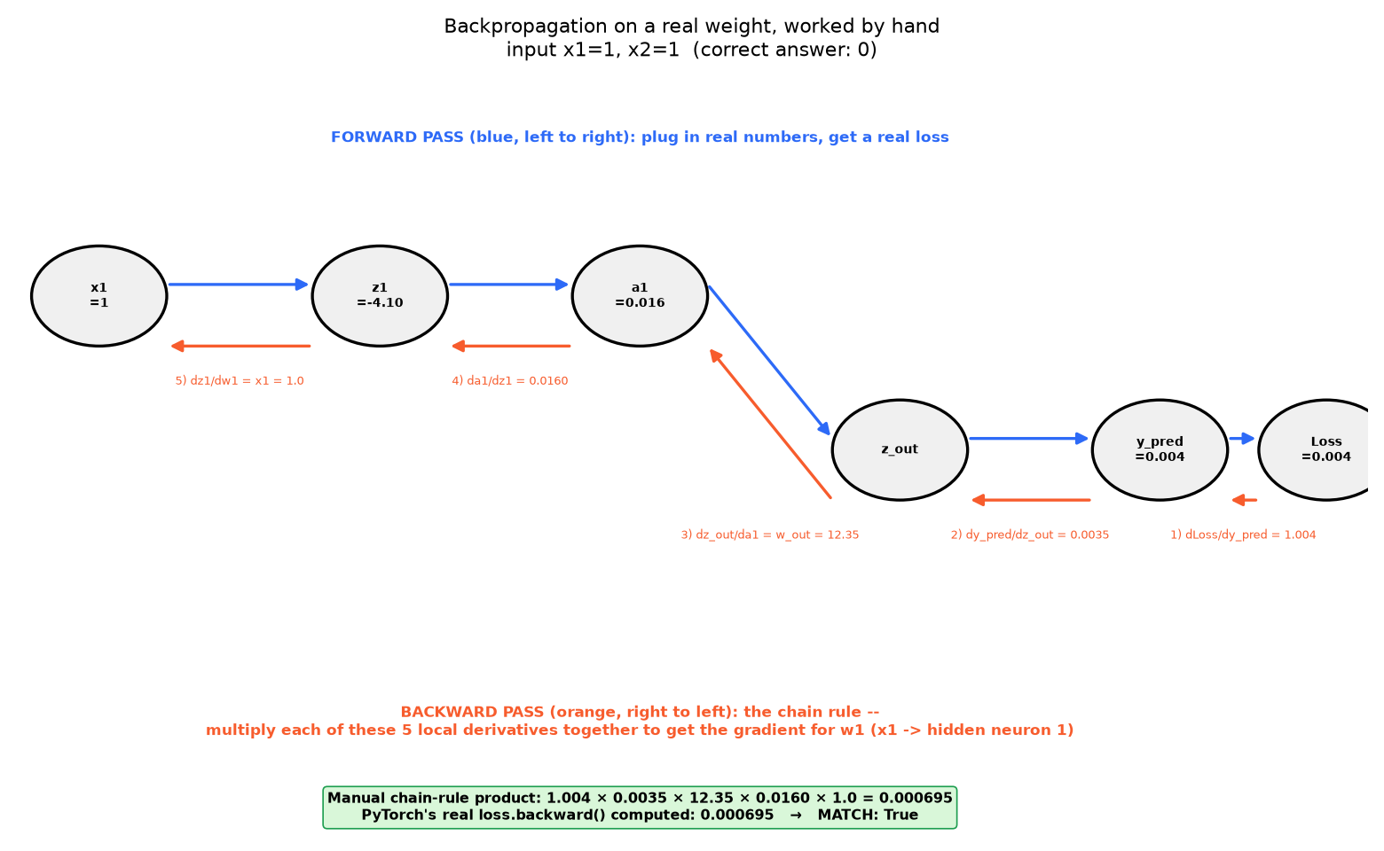
They match exactly — 0.000695 both ways — because they're the same calculation. PyTorch's
autograd isn't doing anything conceptually different from this five-line hand derivation; it's just doing
it automatically, for every single one of the network's weights, every training step.